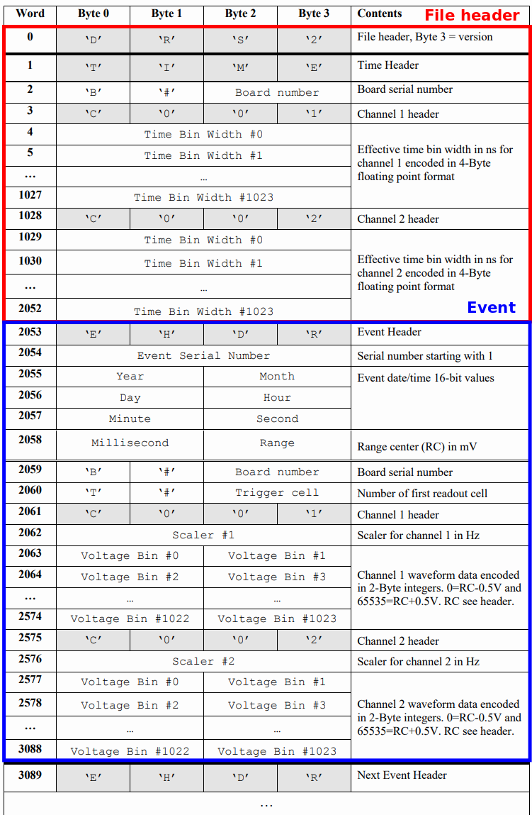
The file header is made of 12+2x(4+1024x4) = 8212 bytes
The event size is 2x(1024x2+8)+32 = 4144 bytes
The bytes can be accessed opening the file as binary open(FILE, 'rb') and read with a usual read().
The struct module in the standard library can be used to unpack data packed in bytes into variables
Example: reading and printing the first 10 bytes (expected charachters "DRS2TIMEB#")
import numpy as np
import struct
f = open('sipm.dat','rb')

head = f.read(10)
print(head)
b'DRS2TIMEB#'
The next 2 bytes contains the board number in a short integer (h)
print(struct.unpack('h', f.read(2))[0])
2528
Then 4 bytes with the channel headers ("COO1" and "C002") and 2 x 1024 floating points (4 bytes each) with the time binnings:
# ch1
ch1 = np.zeros(1024, dtype='float')
print(f.read(4))
for i in range(1024):
    ch1[i] = struct.unpack('f', f.read(4))[0] #  + ch1[i-1] # add the previous value to build the time array

# ch2
ch2 = np.zeros(1024, dtype='float')
print(f.read(4))
for i in range(1024):
    ch2[i] = struct.unpack('f', f.read(4))[0] #  + ch2[i-1]
b'C001'
b'C002'
print(struct.unpack('h', f.read(2))[0])
18501
import matplotlib.pyplot as plt

plt.subplot(221)
plt.plot(ch1)
plt.subplot(222)
plt.plot(ch2)
plt.subplot(223)
plt.hist(ch1, 100)
plt.subplot(224)
plt.hist(ch2, 100)

plt.show()

The total number of events into a single file can be derived from the size.
import os

filesize = os.path.getsize('sipm.dat')
fileheadersize = 12+2*(4+1024*4)
eventsize = 2*(1024*2+8)+32

nevents = int((filesize-fileheadersize)/eventsize)
print('File size:',filesize)
print('File header is',fileheadersize)
print('Single event size is', eventsize)
print('Number of events ->',(filesize-fileheadersize)/eventsize,' rounded:',nevents)
File size: 422612
File header is 8212
Single event size is 4144
Number of events -> 100.0  rounded: 100
But there is a more conveniente way...
In order to import values directly into a structured numpy array, the fromfile() function can be used with proper data types.
Sources/examples:
Header data type (first 8212 bytes):
DRS4header = np.dtype([
    ('timehd', np.dtype('S10')),           # 10 chars
    ('bnr',np.dtype('u2')),                # 2 bytes unsigned integer
    ('ch0head', np.dtype('S4')),           # 4 chars
    ('ch0time', np.dtype(('f', 1024))),   # 1024 x 32bit floating point numbers
    ('ch1head', np.dtype('S4')),           # 4 chars
    ('ch1time', np.dtype(('f', 1024))) ]) # 1024 x 32bit floating point numbers
Read the first 8212 bytes (1 time):
f = open('sipm.dat','rb')
data = np.fromfile(f, dtype=DRS4header, count=1)
plt.hist(data['ch0time'][0], 100, histtype='step', label='ch0 time binning')
plt.hist(data['ch1time'][0], 100, histtype='step', label='ch1 time binning')
plt.xlabel('bin width [ns]')
plt.legend()
plt.show()

Event data type (4144 bytes):
DRS4event = np.dtype([
    ('evhd', np.dtype('S4')),        # 4
    ('srn1',np.dtype('i4')),         # 4 (8)
    ('year',np.dtype('u2')),         # 2 (10)
    ('month',np.dtype('u2')),        # 2 (12)
    ('day',np.dtype('u2')),          # 2 (14)
    ('hour',np.dtype('u2')),         # 2 (16)
    ('minute',np.dtype('u2')),       # 2 (18)
    ('second',np.dtype('u2')),       # 2 (20)
    ('millisec',np.dtype('u2')),     # 2 (22)
    ('range',np.dtype('u2')),        # 2 (24)
    ('boardnrh', np.dtype('S2')),    # 2 (26)
    ('boardnr',np.dtype('u2')),      # 2 (28)
    ('trigcellh', np.dtype('S2')),   # 2 (30)
    ('trigcell',np.dtype('u2')),     # 2 (32)

    ('ch0head', np.dtype('S4')),     # 4 (36)
    ('ch0scaler',np.dtype('i4')),    # 4 (40)
    ('ch0data', np.dtype(('u2', 1024))), # 2x1024 (2088)

    ('ch1head', np.dtype('S4')),     # 4 (2092)
    ('ch1scaler',np.dtype('i4')),    # 4 (2096)
    ('ch1data', np.dtype(('u2', 1024))),  # 2x1024 (4144)

#     ('CH2HEAD', np.dtype('U4')),     # 4 ()
#     ('ch2scaler',np.dtype('i4')),    # 4 ()
#     ('ch2', np.dtype(('u2', 1024))),  # 2x1024 ()

#     ('CH3HEAD', np.dtype('U4')),     # 4 ()
#     ('ch3scaler',np.dtype('i4')),    # 4 ()
#     ('ch3', np.dtype(('u2', 1024)))  # 2x1024 ()
])
f = open('sipm.dat','rb')
head = np.fromfile(f, dtype=DRS4header, count=1)
data = np.fromfile(f, dtype=DRS4event, count=-1)  # count=-1 -> read all the events
print(f"Data start: {data['day'][0]}-{data['month'][0]}-{data['year'][0]} at {data['hour'][0]}:{data['minute'][0]}:{data['second'][0]}")
print(f"Data stop:  {data['day'][-1]}-{data['month'][-1]}-{data['year'][-1]} at {data['hour'][-1]}:{data['minute'][-1]}:{data['second'][-1]}")
print(f"Number of events {data.size}")
Data start: 10-1-2020 at 17:38:35
Data stop:  10-1-2020 at 17:39:12
Number of events 100
Rearrangin data (both time and ADC->V conversion)
ch0time = np.cumsum(head['ch0time'][0])
ch1time = np.cumsum(head['ch1time'][0])
ch0V = data['ch0data']/2**16 - 0.5 + data['range'][0]
ch1V = data['ch1data']/2**16 - 0.5 + data['range'][0]
Check the shape(s):
ch0V.shape, ch1V.shape, ch0time.shape, ch1time.shape
((100, 1024), (100, 1024), (1024,), (1024,))
Plot of 1st event
plt.plot(ch0time, ch0V[0,:])
plt.plot(ch1time, ch1V[0,:])
plt.show()

Overlapping all signals
from matplotlib.colors import LogNorm

fig, ax = plt.subplots(1,2,figsize=(20,5))
ax[0].hist2d(np.tile(ch0time,100),ch0V.flatten(),bins=[1000,100], norm=LogNorm() )
ax[1].hist2d(np.tile(ch1time,100),ch1V.flatten(),bins=[1000,100], norm=LogNorm() )
plt.show()

Trivial analysis
ampli = np.mean(ch0V[:, :100], axis=1) - np.min(ch0V, axis=1)
plt.hist(ampli, bins=50)
plt.show()

maxtime = np.argmin(ch0V, axis=1)

plt.hist2d(maxtime, ampli, bins=20)
plt.show()